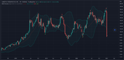
hello everyone, how are you? sorry for insisting on this topic, but this combination of averages really seems to be very promising.
I had already liked Cora Wave a lot and was researching some Jurik indicators on Trading View and I came across this one.
I would like to see how they would look on Renko, but even on candles it already looks interesting. if you can help me to convert at least the Cora Wave, I would be super grateful.
+ if you can kindly include Jurik Composite Fractal Behavior (CFB) on EMA [Loxx], that would be awesome.
Code: Select all
// This source code is subject to the terms of the Mozilla Public License 2.0 at https://mozilla.org/MPL/2.0/
// © loxx

//@version=5
indicator("Jurik Composite Fractal Behavior (CFB) on EMA [Loxx]", shorttitle = "JCFBEMA [Loxx]", overlay = true, timeframe="", timeframe_gaps = true, max_bars_back = 2000)

greencolor = #2DD204
redcolor = #D2042D

EMA(x, t) =>
    _ema = x
    _ema := na(_ema[1]) ? x : (x - nz(_ema[1])) * (2 / (t + 1)) + nz(_ema[1])
    _ema

_jcfbaux(src, depth)=>
    jrc04 = 0.0, jrc05 = 0.0, jrc06 = 0.0, jrc13 = 0.0, jrc03 = 0.0, jrc08 = 0.0
    if (bar_index >= bar_index - depth * 2)
        for k = depth - 1 to 0
            jrc04 += math.abs(nz(src[k]) - nz(src[k+1]))
            jrc05 += (depth + k) * math.abs(nz(src[k]) - nz(src[k+1]))
            jrc06 += nz(src[k+1])
    if(bar_index < bar_index - depth * 2)
        jrc03 := math.abs(src - nz(src[1]))
        jrc13 := math.abs(nz(src[depth]) - nz(src[depth+1]))
        jrc04 := jrc04 - jrc13 + jrc03
        jrc05 := jrc05 - jrc04 + jrc03 * depth
        jrc06 := jrc06 - nz(src[depth+1]) + nz(src[1])
    jrc08 := math.abs(depth * src - jrc06)
    jcfbaux = jrc05 == 0.0 ? 0.0 : jrc08/jrc05
    jcfbaux

_jcfb(src, len, smth) =>
    a1 = array.new<float>(0, 0)
    c1 = array.new<float>(0, 0)
    d1 = array.new<float>(0, 0)
    cumsum = 2.0, result = 0.0

    //crete an array of 2^index, pushed onto itself
    //max values with injest of depth = 10: [1, 1, 2, 2, 4, 4, 8, 8, 16, 16, 32, 32, 64, 64, 128, 128, 256, 256, 512, 512]
    for i = 0 to len -1
        array.push(a1, math.pow(2, i))
        array.push(a1, math.pow(2, i))

    //cumulative sum of 2^index array
    //max values with injest of depth = 10: [2, 3, 4, 6, 8, 12, 16, 24, 32, 48, 64, 96, 128, 192, 256, 384, 512, 768, 1024, 1536]
    for i = 0 to array.size(a1) - 1
        array.push(c1, cumsum)
        cumsum += array.get(a1, i)

    //add values from jcfbaux calculation using the cumumulative sum arrary above
    for i = 0 to array.size(c1) - 1
        array.push(d1, _jcfbaux(src, array.get(c1, i)))

    baux = array.copy(d1)
    cnt = array.size(baux)
    arrE = array.new<float>(cnt, 0)
    arrX = array.new<float>(cnt, 0)

    if bar_index <= smth
        for j = 0 to bar_index - 1
            for k = 0 to cnt - 1
                eget = array.get(arrE, k)
                array.set(arrE, k, eget + nz(array.get(baux, k)[bar_index - j]))
        for k = 0 to cnt - 1
            eget = nz(array.get(arrE, k))
            array.set(arrE, k, eget / bar_index)
    else
        for k = 0 to cnt - 1
            eget = nz(array.get(arrE, k))
            array.set(arrE, k, eget + (nz(array.get(baux, k)) - nz(array.get(baux, k)[smth])) / smth)
    if bar_index > 5
        a = 1.0, b = 1.0
        for k = 0 to cnt - 1
            if (k % 2 == 0)
                array.set(arrX, k, b * nz(array.get(arrE, k)))
                b := b * (1 - nz(array.get(arrX, k)))
            else
                array.set(arrX, k, a * nz(array.get(arrE, k)))
                a := a * (1 - nz(array.get(arrX, k)))
        sq = 0.0, sqw = 0.0
        for i = 0 to cnt - 1
            sqw += nz(array.get(arrX, i)) * nz(array.get(arrX, i)) * nz(array.get(c1, i))
        for i = 0 to array.size(arrX) - 1
            sq += math.pow(nz(array.get(arrX, i)), 2)
        result := sq == 0.0 ? 0.0 : sqw / sq
        result

_a_jurik_filt(src, len, phase) =>
    //static variales
    volty = 0.0, avolty = 0.0, vsum = 0.0, bsmax = src, bsmin = src
    len1 = math.max(math.log(math.sqrt(0.5 * (len-1))) / math.log(2.0) + 2.0, 0)
    len2 = math.sqrt(0.5 * (len - 1)) * len1
    pow1 = math.max(len1 - 2.0, 0.5)
    beta = 0.45 * (len - 1) / (0.45 * (len - 1) + 2)
    div = 1.0 / (10.0 + 10.0 * (math.min(math.max(len-10, 0), 100)) / 100)
    phaseRatio = phase < -100 ? 0.5 : phase > 100 ? 2.5 : 1.5 + phase * 0.01
    bet = len2 / (len2 + 1)

    //Price volatility
    del1 = src - nz(bsmax[1])
    del2 = src - nz(bsmin[1])
    volty := math.abs(del1) > math.abs(del2) ? math.abs(del1) : math.abs(del2)

    //Relative price volatility factor
    vsum := nz(vsum[1]) + div * (volty - nz(volty[10]))
    avolty := nz(avolty[1]) + (2.0 / (math.max(4.0 * len, 30) + 1.0)) * (vsum - nz(avolty[1]))
    dVolty = avolty > 0 ? volty / avolty : 0
    dVolty := math.max(1, math.min(math.pow(len1, 1.0/pow1), dVolty))

    //Jurik volatility bands
    pow2 = math.pow(dVolty, pow1)
    Kv = math.pow(bet, math.sqrt(pow2))
    bsmax := del1 > 0 ? src : src - Kv * del1
    bsmin := del2 < 0 ? src : src - Kv * del2

    //Jurik Dynamic Factor
    alpha = math.pow(beta, pow2)

    //1st stage - prelimimary smoothing by adaptive EMA
    jma = 0.0, ma1 = 0.0, det0 = 0.0, e2 = 0.0
    ma1 := (1 - alpha) * src + alpha * nz(ma1[1])

    //2nd stage - one more prelimimary smoothing by Kalman filter
    det0 := (src - ma1) * (1 - beta) + beta * nz(det0[1])
    ma2 = ma1 + phaseRatio * det0

    //3rd stage - final smoothing by unique Jurik adaptive filter
    e2 := (ma2 - nz(jma[1])) * math.pow(1 - alpha, 2) + math.pow(alpha, 2) * nz(e2[1])
    jma := e2 + nz(jma[1])
    jma


src = input.source(hlcc4, "Source", group = "Basic Settings")

cfb_src = input.source(hlcc4, "CFB Source", group = "CFB Ingest Settings")

// backsamping period for highs/lows
nlen = input.int(50, "CFB Normal Length", minval = 1, group = "CFB Ingest Settings")

// cfb depth, max 10 since that's around 5000 bars
cfb_len = input.int(10, "CFB Depth", maxval = 10, group = "CFB Ingest Settings")

// internal cfb calc smoothing
smth = input.int(8, "CFB Smooth Length", minval = 1, group = "CFB Ingest Settings")

 // lower bound of samples returned from the nlen rolling window
slim = input.int(10, "CFB Short Limit", minval = 1, group = "CFB Ingest Settings")

// upper bound of samples returned from the nlen rolling window
llim = input.int(20, "CFB Long Limit", minval = 1, group = "CFB Ingest Settings")

// for jurik filter post cfb calcuation smoothing length
jcfbsmlen = input.int(10, "CFB Jurik Smooth Length", minval = 1, group = "CFB Ingest Settings")

// for jurik filter post cfb calcuation smoothing phase, generall a number between -100 and 100
jcfbsmph = input.float(0, "CFB Jurik Smooth Phase", group = "CFB Ingest Settings")


colorbars = input.bool(true, title='Color bars?', group = "UI Options")


cfb_draft = _jcfb(cfb_src, cfb_len, smth)
cfb_pre = _a_jurik_filt(_a_jurik_filt(cfb_draft, jcfbsmlen, jcfbsmph), jcfbsmlen, jcfbsmph)

max = ta.highest(cfb_pre, nlen)
min = ta.lowest(cfb_pre, nlen)
denom = max - min
ratio = (denom > 0) ? (cfb_pre - min) / denom : 0.5
len_out_cfb = math.ceil(slim + ratio * (llim - slim))

emaout = EMA(src, int(len_out_cfb))

plot(emaout, color = src >= emaout ? greencolor : redcolor, linewidth = 3)

barcolor(color = src >= emaout ? greencolor : redcolor)
Code: Select all
//@version=4
// This source code is subject to the terms of the Mozilla Public License 2.0 at https://mozilla.org/MPL/2.0/
// © RedKTrader

study("Comp_Ratio_MA", shorttitle = "CoRa Wave", overlay = true, resolution ="")

// ======================================================================
// Compound Ratio Weight MA function
// Compound Ratio Weight is where the weight increases in a "logarithmicly linear" way (i.e., linear when plotted on a log chart) - similar to compound ratio
// the "step ratio" between weights is consistent - that's not the case with linear-weight moving average (WMA), or EMA
// another advantage is we can significantly reduce the "tail weight" - which is "relatively" large in other MAs and contributes to lag
//
// Compound Weight ratio     r = (A/P)^1/t - 1
// Weight at time t         A = P(1 + r)^t
//                            = Start_val * (1 + r) ^ index
// Note: index is 0 at the furthest point back -- num periods = length -1
//
f_adj_crwma(source, length, Start_Wt, r_multi) =>
    numerator = 0.0, denom = 0.0, c_weight = 0.0
    //Start_Wt = 1.0    // Start Wight is an input in this version - can also be set to a basic value here.
    End_Wt = length     // use length as initial End Weight to calculate base "r"
    r = pow((End_Wt / Start_Wt),(1 / (length - 1))) - 1
    base = 1 + r * r_multi
    for i = 0 to length -1
        c_weight    := Start_Wt * pow(base,(length - i))
        numerator   := numerator + source[i] * c_weight
        denom       := denom + c_weight
    numerator / denom
// ====================================================================== ==

data        = input(title = "Source",                 type = input.source,      defval = hlc3)
length      = input(title = "length",                 type = input.integer,     defval = 20,  minval = 1)
r_multi     = input(title = "Comp Ratio Multiplier",  type = input.float,       defval = 2.0, minval = 0, step = .1)
smooth      = input(title = "Auto Smoothing",         type = input.bool,        defval = true,                    group = "Smoothing")
man_smooth  = input(title = "Manual Smoothing",       type = input.integer,     defval = 1, minval = 1, step = 1, group = "Smoothing")

s           = smooth ? max(round(sqrt(length)),1) : man_smooth
cora_raw    = f_adj_crwma(data, length, 0.01, r_multi)
cora_wave   = wma(cora_raw, s)

c_up        = color.new(color.aqua, 0)
c_dn        = color.new(#FF9800   , 0)
cora_up     = cora_wave > cora_wave[1]
plot(cora_wave, title="Adjustible CoRa_Wave", color = cora_up ? c_up : c_dn, linewidth = 3)